- Order of estimation: Size → Effort → Schedule. COCOMO turns size into effort and then into time.
- COCOMO (slides 37–51) is the calculation part; methods (9–17) are the written-answer part.
- Why hard: evolving requirements, technical unknowns, team skill/availability, external dependencies.
- Basic process: size → effort (person-months) → schedule.
🎯 How this can come up · 1 question
What is the correct order of the basic estimation process?
Correct: Size → effort → schedule.
- No exact estimate exists. Software estimates are commonly off by 25–100%.
- Target date = from business/marketing. Committed date = what the team agrees after planning. Don’t commit to targets early.
- Bigger project → more variance (7% small … 51% very large).
🎯 How this can come up · 1 question
A target date is one the team commits to after building a schedule.
False. That is a committed date. Targets come from business or marketing.
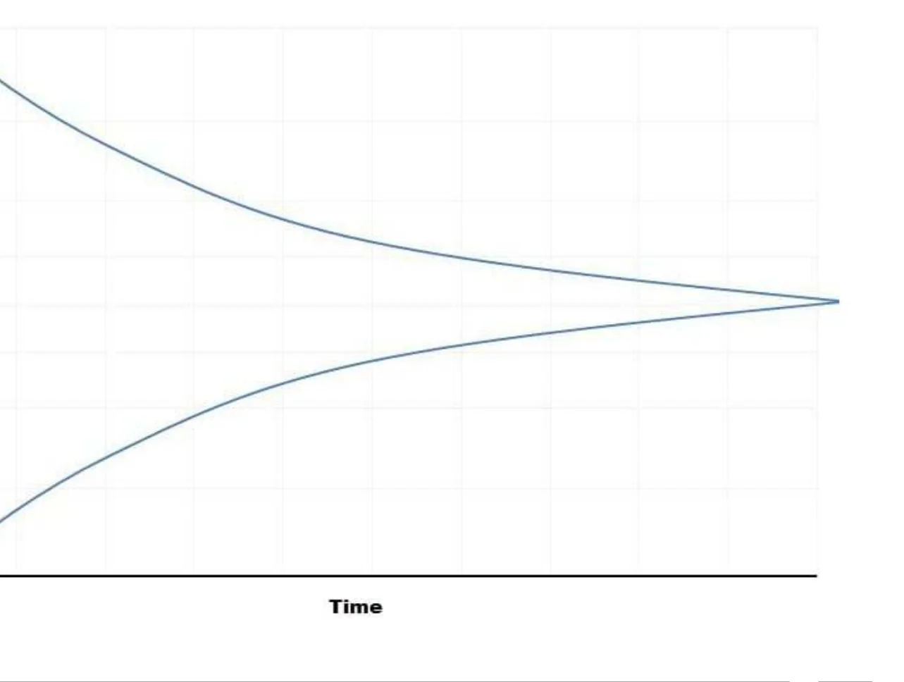
- Early estimates can be 0.25× to 4× the real value; the cone narrows as you learn.
🎯 How this can come up · 1 question
At the feasibility stage, the cone of uncertainty says estimates may range from:
Correct: 0.25x to 4x.
- Six methods. In an exam scenario, pick two and say WHY they fit (e.g., analogy early using past projects; bottom-up once a WBS exists).
Asked in a real exam
🎯 How this can come up · 1 question
Choose two effort-estimation techniques for a 12-month hardware/software project and explain how each supports planning and risk control (Final 242).
Bottom-up estimation: decompose the work into a WBS and estimate each task with the people who will do it; this is the most accurate, exposes hidden work and gives a baseline to track against. Three-point (PERT) estimating: for uncertain tasks like prototyping, get optimistic, most likely and pessimistic values and compute (O+4M+P)/6; the spread shows risk and sizes contingency reserves. Alternatives: analogy to past solar projects early on, Wideband Delphi for expert consensus, COCOMO for the software part. Validate estimates by comparing two methods and against historical data, and refine iteratively.
- Expert judgment = a “guesstimate”; only as good as the expert’s real experience.
- Top-down: quick, good early; less accurate (misses task complexity).
- Bottom-up: from the WBS up; most accurate but slow and needs detail.
🎯 How this can come up · 1 question
Which method requires a work breakdown structure and is the most granular?
Correct: Bottom-up.
- Analogy: compare with a similar past project. Hard to match projects exactly.
- Priced to win = estimate driven by the price that wins the bid, not the real effort. Risk of underbidding and overruns.
- Algorithmic size measures: LOC and function points mostly.
- Wideband Delphi: independent estimates → discussion → anonymous re-estimates → repeat until consensus.
- No historical data needed; may still converge on a shared bias.
🎯 How this can come up · 1 question
Wideband Delphi requires historical project data.
False. It does not; it uses several experts.
- LOC: easy to count afterwards, hard to estimate early; varies by language; easy to game.
- Function points size software by its functions, independent of language.
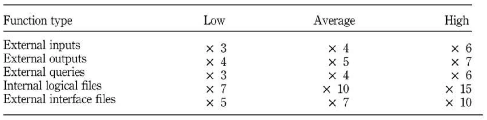
- FP steps: count functions (inputs, outputs, inquiries, files, interfaces) → weight by complexity → UFP → multiply by influence factor (14 factors, 0–5).
🎯 How this can come up · 1 question
How many influence factors adjust the function point count?
Correct: 14.
- From size to effort: empirical, mathematical (Effort = a × Sizeb), or subjective models.
- Duration = calendar working days. Effort = labor (staff-hours). 5 people × 10 h = 50 staff-hours of effort but 10 h of duration.
🎯 How this can come up · 1 question
Five people review a document for 10 hours. Effort and duration are:
Correct: 50 staff-hours effort, 10 hours duration.
- Productivity is only 50–75% of the day, so 40 labor hours need ~50+ clock hours.
- Variation: skill levels, unexpected events, interruptions, rework.
- Good data comes at the end; save it for the next project.
- Overestimate → not funded, Parkinson’s law (work fills the time), scope creep. Underestimate → cut testing, missed deadlines, low morale.
🎯 How this can come up · 1 question
“Work expands to fill the time available” is:
Correct: Parkinson’s Law.
- Resource estimation = who/what, how much, when.
Related real-exam questions
- Controlling factors: environment, organization policy, availability.
- Tools: expert judgment, alternatives analysis (in-house vs contract vs COTS), published data.
- Outputs: resource requirements per activity, resource calendar, change requests.
- Duration estimates come from those who know the work, and improve over time.
- More people can lower productivity (Mythical Man-Month, Chapter 6.2).
Seen again
- Keep one time unit; convert at the end.
- Contingency (buffer) time ≠ slack. Buffer is added on purpose; slack comes from the network.
- Basic three-point = (M + O + P) / 3.
Seen again
- PERT/beta formula: (O + 4M + P) / 6 weights the most likely value 4×.
🎯 How this can come up · 2 questions
O = 4 days, M = 6 days, P = 14 days. PERT estimate?
(4 + 24 + 14) / 6 = 42/6 = 7.
O = 2, M = 5, P = 8. Basic (simple average) three-point estimate?
(2+5+8)/3 = 5.
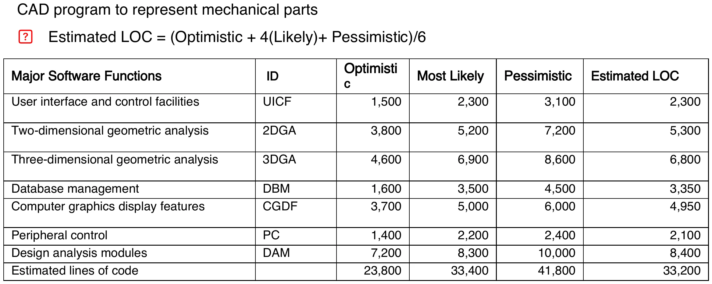
- Example: UICF (1,500 + 4×2,300 + 3,100)/6 = 2,300. Totals give 33,200 LOC.
- Weights (low/average/high): inputs 3/4/6, outputs 4/5/7, queries 3/4/6, internal files 7/10/15, external interfaces 5/7/10.
- COCOMO: input KLOC → output person-months.
- Biggest weakness: needs a reliable LOC estimate up front.
🎯 How this can come up · 1 question
The biggest weakness of COCOMO is that it:
Correct: Requires a reliable size (LOC) estimate as input.
- Effort E = a × KLOCb (person-months).
- a, b → effort. c, d → time.
- Organic 2–50 KLOC · Semi-detached 50–300 · Embedded >300 or severe constraints.
- Note c = 2.5 for all three modes.
🎯 How this can come up · 2 questions
Which COCOMO mode has a = 3.0 and b = 1.12?
Correct: Semi-detached.
In Basic COCOMO, c = 2.5 for all three modes.
True.
- Same size, more complex mode → much more effort (626 → 2,077).
- Time TDEV = c × Ed (months). Uses E, not KLOC.
- Interesting: all three give ~29 months. Harder projects need more PEOPLE, not more time.
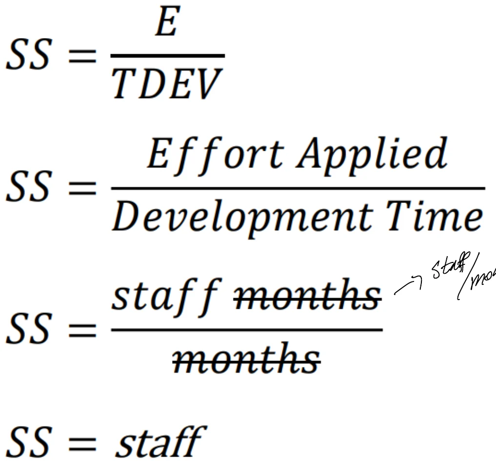
- Average staff SS = E / TDEV.
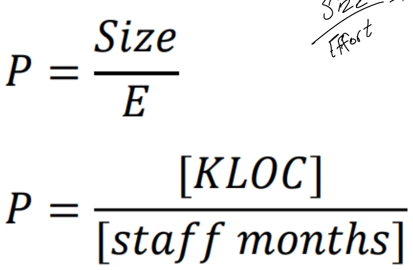
- Productivity P = Size / E (LOC per person-month).
- The full recipe: E → TDEV → SS = E/TDEV → P = LOC/E. Exactly what both finals asked.
Asked in a real exam
🎯 How this can come up · 2 questions
COCOMO organic, 32 KLOC (a=2.4, b=1.05, c=2.5, d=0.38). Compute effort, development time and average staff (Final 242).
E = 2.4 × 32^1.05 ≈ 2.4 × 38.06 ≈ 91.3 person-months. TDEV = 2.5 × 91.3^0.38 ≈ 2.5 × 5.56 ≈ 13.9 months. Average staff = E / TDEV ≈ 91.3 / 13.9 ≈ 6.6 people (about 7).
COCOMO organic, 20 KLOC. Compute effort, development time, productivity and staff (Final 251).
E = 2.4 × 20^1.05 ≈ 2.4 × 23.2 ≈ 55.8 person-months. TDEV = 2.5 × 55.8^0.38 ≈ 2.5 × 4.61 ≈ 11.5 months. Productivity = 20,000 LOC / 55.8 PM ≈ 359 LOC per person-month. Staff = 55.8 / 11.5 ≈ 4.8 people (about 5).
- Answer to “Conclusion ?”: an embedded project needs far more effort per line, so expected productivity is only ~127 LOC per person-month (vs 375 organic).
🎯 How this can come up · 1 question
An organic project is estimated at E = 40 PM and TDEV = 10 months. Average staff?
SS = E / TDEV.
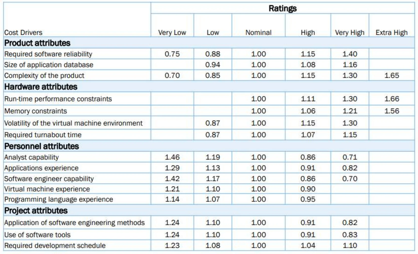
- Intermediate COCOMO: 15 cost drivers adjust effort (product, hardware, personnel, project attributes).
- C = product of all cost-driver multipliers; E = a × KLOCb × C.
🎯 How this can come up · 1 question
In Intermediate COCOMO the cost-driver multipliers are added together.
False. They are multiplied; the product is C.
- Pros: history-based, repeatable, modes, calibrated, documented, easy.
- Cons: ignores volatility, documentation, customer skill, turnover, safety… and still needs a size estimate.
- Reuse isn’t free: reused ≈ 30% of new effort, modified ≈ 60%, >50% modified = new.
- Agile: story → tasks → estimate each → sum → increment estimate.
- Real deadlines tie to external events; artificial ones may flex.
- Present estimates with uncertainty: ±, ranges, risk quantification, cases, coarse dates, confidence factors.
🎯 How this can come up · 1 question
“July 1 with 50% probability” is which presentation technique?
Correct: Confidence factors.
- Contingency → PM controls; management reserve → needs change control to use.
- Estimate iteratively, refining as you learn.
- Allow for non-project time and junior staff.
- Student syndrome = procrastinate until the last minute, so padding gets wasted.
🎯 How this can come up · 1 question
Team members who wait until the last minute to start a task despite padding show:
Correct: Student syndrome.
No slides match this filter.